使用SVM对鸢尾花分类
使用SVM对鸢尾花分类
百度AI Studio中的一个入门项目,增加了自己在实践时的一些注释,对小白来说阅读更顺畅。源码和数据在github上。
任务描述:
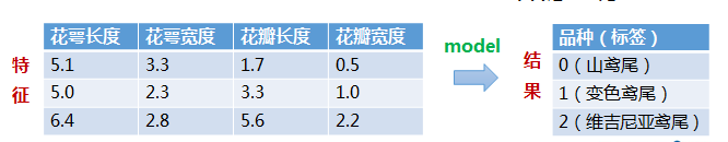
构建一个模型,根据鸢尾花的花萼和花瓣大小将其分为三种不同的品种。
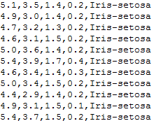
数据集
总共包含150行数据
每一行数据由 4 个特征值及一个目标值组成。
4 个特征值分别为:萼片长度、萼片宽度、花瓣长度、花瓣宽度
目标值为三种不同类别的鸢尾花,分别为: Iris Setosa、Iris Versicolour、Iris Virginica
首先导入必要的包:
numpy:python第三方库,用于科学计算
matplotlib:python第三方库,主要用于进行可视化
sklearn:python的重要机器学习库,其中封装了大量的机器学习算法,如:分类、回归、降维以及聚类
1 | import numpy as np |
Step1.数据准备
(1)从指定路径下加载数据
(2)对加载的数据进行数据分割,x_train,x_test,y_train,y_test分别表示训练集特征、训练集标签、测试集特征、测试集标签
1 | #*************将字符串转为整型,便于数据加载*********************** |
1 | #加载数据 |
random_state=1确保了每次运行程序时用的随机数都是一样的,也就是每次重新运行后所划分的训练集和测试集的样本都是一致的,相当于只在第一次运行的时候进行随机划分。如果不设置的话,每次重新运行的种子不一样,产生的随机数也不一样就会导致每次随机生成的训练集和测试集不一致。
Step2.模型搭建
C越大,相当于惩罚松弛变量,希望松弛变量接近0,即对误分类的惩罚增大,趋向于对训练集全分对的情况,这样对训练集测试时准确率很高,但泛化能力弱。
C值小,对误分类的惩罚减小,允许容错,将他们当成噪声点,泛化能力较强。
kernel=’linear’时,为线性核
decision_function_shape=’ovr’时,为one v rest,即一个类别与其他类别进行划分,
decision_function_shape=’ovo’时,为one v one,即将类别两两之间进行划分,用二分类的方法模拟多分类的结果。
ovr是多类情况1和ovo是多类情况2,可以在我个人博客-线性判别函数 上查看详细说明。
1 | #**********************SVM分类器构建************************* |
1 | # 2.定义模型:SVM模型定义 |
Step3.模型训练
1 | y_train.ravel()#ravel()扁平化,将原来的二维数组转换为一维数组 |
1 | array([2., 0., 0., 0., 1., 0., 0., 2., 2., 2., 2., 2., 1., 2., 1., 0., 2., |
1 | #***********************训练模型***************************** |
1 | # 3.训练SVM模型 |
Step4.模型评估
1 | #**************并判断a b是否相等,计算acc的均值************* |
1 | def print_accuracy(clf,x_train,y_train,x_test,y_test): |
1 | # 4.模型评估 |
1 | trianing prediction:0.819 |
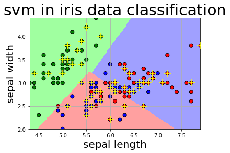
Step5.模型使用
np.mgrid的作用是用前两个特征生成其对应最大最小范围所能组合出的所有200*200的样本,也就是遍历了这两个特征所能组合出的所有可能性,只是粒度是1/200
1 | def draw(clf, x): |
1 | # 5.模型使用 |
1 | grid_test: |